Simple models
(Marcello Gallucci)
keywords multiple regression, path analysis, lavaan, multivatiate regression
Draft version, mistakes may be around
In this example we show how to estimate simple regression models with
PATHj. The aim is threefold: first, it
may help seeing how the SEM module can estimate path analysis, and see
how path analysis encompasses models usually estimated with the General
Linear Model (but look at GAMLj
module for a specialized module in jamovi). Second, we are going to estimate some
models discussed in UCLA statistical
consulting webpage, so one can compare the results obtained in
lavaan with the ones obtained in PATHj. Third, we show how to add some
interesting test and twist to simple regression models.
Much of the output that PATHj produces is labeled as it is in lavaan R package output, so lots of information can be found in lavaan help and tutorials
Research data
The data we use can be found here at UCLA. The sample is composed by 500 students, each with 9 observed variables: Motivation (motiv), Harmony (harm), Stability (stabi), Negative Parental Psychology (ppsych), SES, Verbal IQ (verbal), Reading (read), Arithmetic (arith) and Spelling (spell). They are all continuous variables.
Simple regression (Model 1A)
First, we estimate a simple regression with read as dependent (endogenous) variable and motiv as independent (exogenous) variable.
Input
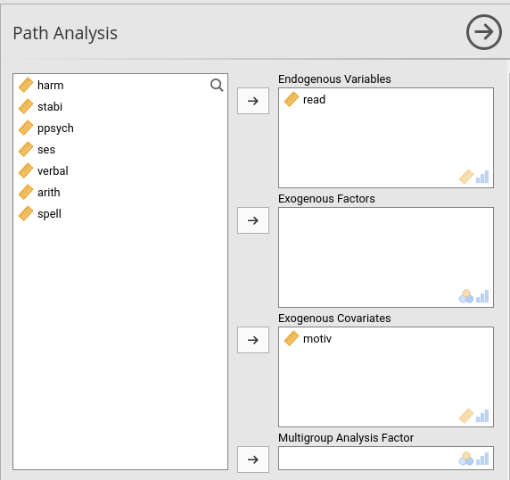
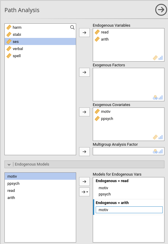
In PATHj we set the variables roles in the first panel as shown here: The dependent variable goes in the Endogenous Variables field, and the independent variable goes in the Exogenous Variables field.
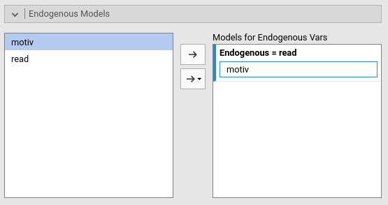
Then we specify the endogenous variable predictor in the Endogenous Models panel
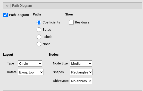
Because we want to see the path diagram of the model (although in this case is too simple to be interesting), we ask for the path diagram in the Path Diagram panel.
Output
General info
 Models Info
 ─────────────────────────────────────────────────────────

 ─────────────────────────────────────────────────────────
   Estimation Method                   ML              .
   Number of observations              500
   Free parameters                     3
   Converged                           TRUE

   Loglikelihood user model            -1777.823
   Loglikelihood unrestricted model    -1777.823

   Model                               read ~ motiv
 ─────────────────────────────────────────────────────────
The first table we obtain informs us about the sample size, the model
we run, and the log-likelihood. We have 500 cases, upon which we
estimated the read~motiv model, which requires 3 free
parameters: The effect of motiv on read, the
variance of read and the intercept.
Loglikelihood user model and
Loglikelihood unrestricted model are the same and indicate
the log likelihood of the model. They are the same because we did not
restrict any parameter, so the user model is the unrestricted model.
Overall tests
 OVERALL TESTS

 Model Tests
 ──────────────────────────────────────────────────
   Label             X²          df    p
 ──────────────────────────────────────────────────
   Baseline Model    164.8774     1    < .0000001
 ──────────────────────────────────────────────────


 Fit Indices
 ─────────────────────────────────────────────────────────────────────────────────────────────────────
   AIC         BIC         adj. BIC    SRMR         RMSEA        Lower        Upper        RMSEA p
 ─────────────────────────────────────────────────────────────────────────────────────────────────────
   3561.645    3574.289    3564.767    0.0000001    0.0000000    0.0000000    0.0000000
 ─────────────────────────────────────────────────────────────────────────────────────────────────────


 Fit Indices
 ──────────────────────────────────────────────────────────────────────────────
   CFI          TLI          RNI          GFI          adj. GFI     pars. GFI
 ──────────────────────────────────────────────────────────────────────────────
   1.0000000    1.0000000    1.0000000    1.0000000    1.0000000    0.0000000
 ──────────────────────────────────────────────────────────────────────────────
Model tests table reports the chi-square of the whole
model. Because there is no fixed parameter, the model chi-square is
zero, and it is not shown. The Baseline model row refers to
the comparison between the user model, that is read~motiv,
and a model in which the variables covariance is set to zero. In this
case, it is simply testing that the effect of motiv on
read is different from zero.
Fit indices are the standard indices reported is structural equation models.
\(R^2\)
The \(R^2\) and its’ confidence interval is reported. For details about the C.I. estimation, please refer to PATHj computation details
Coefficients
 Parameter Estimates
 ─────────────────────────────────────────────────────────────────────────────────────────────────────────────
   Dep     Pred     Estimate     SE            Lower        Upper        β            z           p
 ─────────────────────────────────────────────────────────────────────────────────────────────────────────────
   read    motiv    0.5300000    0.03792361    0.4556711    0.6043289    0.5300000    13.97546    < .0000001
 ─────────────────────────────────────────────────────────────────────────────────────────────────────────────
The Parameter Estimates table reports the regression
coefficients. Notice that the Estimate is the B
coefficient, and the \(\beta\) is the
fully standardized coefficient. In this case they are equal because the
variables have the same variance (100), which implies that B and \(\beta\) are equal.
Additional parameters
 Variances and Covariances
 ──────────────────────────────────────────────────────────────────────────────────────────────────────────────────────────────────────────
   Variable 1    Variable 2    Estimate    SE          Lower       Upper       β            z           p             Method    Type
 ──────────────────────────────────────────────────────────────────────────────────────────────────────────────────────────────────────────
   read          read          71.76618    4.538892    62.87012    80.66225    0.7191000    15.81139    < .0000001    Estim     Residuals
   motiv         motiv         99.80000    0.000000    99.80000    99.80000    1.0000000                              Sample    Variables
 ──────────────────────────────────────────────────────────────────────────────────────────────────────────────────────────────────────────
The Variances and Covariances table reports variables
estimated parameters. As regards read, we obtain the
estimated residual variance (cf. columns Type and
Method). For motiv, we obtain the whole
variance computed in the sample. This happens because, by
default, PATHj assumes the exogenous
variables to be fixed variables, like in standard regression. This is
usually a good idea, but in case one wants to estimate also the
variances of the exogenous variables, one can unselect the option Parameters Options -> Fixed Exogenous.
Alternatively, one can estimate this variance by specifying in Custom Model Setting the code
motive~~motive.
The Intercepts table reports the intercepts. Coherently
with the fact that the variables are centered to their means in the
original data-set, all intercepts are 0.
 Intercepts
 ───────────────────────────────────────────────────────────────────────────────────────────
   Variable    Intercept    SE           Lower         Upper        z            p
 ───────────────────────────────────────────────────────────────────────────────────────────
   read        0.0000000    0.3788567    -0.7425454    0.7425454    0.0000000    1.0000000
   motiv       0.0000002    0.0000000     0.0000002    0.0000002
 ───────────────────────────────────────────────────────────────────────────────────────────
These results, in terms of coefficients and \(R^2\), are equivalent to the results one would obtain with a standard OLS regression.
Multiple regression (Model 2)
Input
In model 2 we add a second predictor ppsych, first in
the variables role panel, then to the endogenous variables model.

Output
Results are in line with a standard multiple regression model. The path diagram is as follows

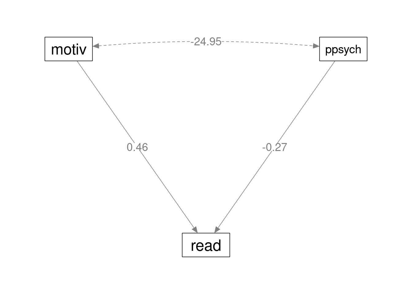
We do not go through the output again, because we would find the same
tables with the same interpretation as before. However, we can do
something with this model that OLS regression does not allow to do with
simplicity. We test the null-hypothesis that the two predictors have the
same effect. In other words, we test that the effect from
motiv to read is not different from the effect
from ppsych to read.
Let’s look at the parameters we have just estimated.
 Parameter Estimates
 ───────────────────────────────────────────────────────────────────────────────────────────────────────────────────
   Dep     Pred      Estimate      SE            Lower         Upper         β             z            p
 ───────────────────────────────────────────────────────────────────────────────────────────────────────────────────
   read    motiv      0.4613333    0.03719135     0.3884396     0.5342270     0.4613333    12.404318    < .0000001
   read    ppsych    -0.2746667    0.03719135    -0.3475604    -0.2017730    -0.2746667    -7.385230    < .0000001
 ───────────────────────────────────────────────────────────────────────────────────────────────────────────────────
 Variances and Covariances
 ──────────────────────────────────────────────────────────────────────────────────────────────────────────────────────────────────────────────
   Variable 1    Variable 2    Estimate     SE          Lower        Upper        β             z           p             Method    Type
 ──────────────────────────────────────────────────────────────────────────────────────────────────────────────────────────────────────────────
   read          read           64.70766    4.092472     56.68656     72.72876     0.6483733    15.81139    < .0000001    Estim     Residuals
   motiv         motiv          99.80000    0.000000     99.80000     99.80000     1.0000000                              Sample    Variables
   motiv         ppsych        -24.95000    0.000000    -24.95000    -24.95000    -0.2500000                              Sample    Variables
   ppsych        ppsych         99.80000    0.000000     99.80000     99.80000     1.0000000                              Sample    Variables
 ──────────────────────────────────────────────────────────────────────────────────────────────────────────────────────────────────────────────
We want to test the null-hypothesis .461=-.275. This test makes sense
because the two coefficients have the same scale, as indicated by the
fact that motiv and ppsych have the same
variance (see Variances and Covariances table).
To obtain this test, we need to restrict the two coefficients to be equal. We go to Custom Model Settings and flag the option Show parameters labels.
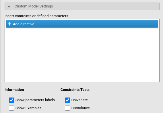
Parameters labels are shortcuts to refer to a coefficient used in
lavaan syntax. PATHj assigns
automatically a label to each parameter from p1 to
pk, where k is the number of parameters in the
model. Parameters labels are shown in the tables.
 Parameter Estimates
 ────────────────────────────────────────────────────────────────────────────────────────────────────────────────────────────
   Label    Dep     Pred      Estimate      SE            Lower         Upper         β             z            p
 ────────────────────────────────────────────────────────────────────────────────────────────────────────────────────────────
   p1       read    motiv      0.4613333    0.03719135     0.3884396     0.5342270     0.4613333    12.404318    < .0000001
   p2       read    ppsych    -0.2746667    0.03719135    -0.3475604    -0.2017730    -0.2746667    -7.385230    < .0000001
 ────────────────────────────────────────────────────────────────────────────────────────────────────────────────────────────
We see in the table that the two coefficients that are interesting us are labeled p1 and p2. Thus, we go to the Custom Model Settings panel and constraints them as equal.
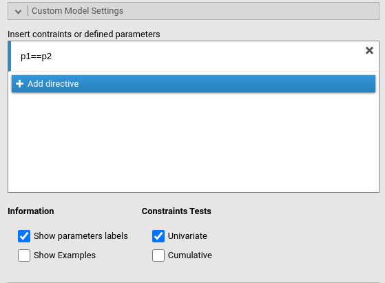
The output now reports the coefficients as equal to .093.
 Parameter Estimates
 ─────────────────────────────────────────────────────────────────────────────────────────────────────────────────────────
   Label    Dep     Pred      Estimate      SE            Lower         Upper        β             z           p
 ─────────────────────────────────────────────────────────────────────────────────────────────────────────────────────────
   p1       read    motiv     0.09333336    0.03627549    0.02223470    0.1644320    0.09333336    2.572904    0.0100849
   p2       read    ppsych    0.09333336    0.03627549    0.02223470    0.1644320    0.09333335    2.572904    0.0100849
 ─────────────────────────────────────────────────────────────────────────────────────────────────────────────────────────
In the output we also find a new table,
Constraints Score Tests, which provides a chi-square test
comparing the original model with the constrained model with the two
coefficients set as equal. The test null-hypothesis is that they are
equal, thus if one finds the test to be significant, one can
reject the null-hypothesis. In this case, the coefficients can be
considered as statistically different.
 Constraints Score Tests
 ──────────────────────────────────────────────────────────────────────
   Type          Par 1          Par 2    X²          df    p
 ──────────────────────────────────────────────────────────────────────
   Univariate    p1       ==    p2       171.5212     1    < .0000001
 ──────────────────────────────────────────────────────────────────────
We the same logic, one can test any reasonable hypothesis in a model by restricting the appropriate coefficients to be equal or to equate a specific value.
Multivariate regression
(Models 3A-E)
We can now add some endogenous dependent variables. We add
arith (arithmetic test score) as dependent
variable in the model, with motiv and ppsych
as predictors of read, and only motiv as
predictor of arith. The path diagram looks like this.

We obtain this model by adding arith to the Endogeneous Variables field, and then defining its
predictor in the Endogenous Models
panel.
We get exactly the same results obtained in lavaan (cf UCLA statistical consulting webpage).
 Parameter Estimates
 ────────────────────────────────────────────────────────────────────────────────────────────────────────────────────
   Dep      Pred      Estimate      SE            Lower         Upper         β             z            p
 ────────────────────────────────────────────────────────────────────────────────────────────────────────────────────
   read     motiv      0.4760551    0.03685137     0.4038277     0.5482824     0.4818294    12.918245    < .0000001
   read     ppsych    -0.2157797    0.02960409    -0.2738027    -0.1577568    -0.2183970    -7.288849    < .0000001
   arith    motiv      0.6000000    0.03577709     0.5298782     0.6701218     0.6000000    16.770508    < .0000001
 ────────────────────────────────────────────────────────────────────────────────────────────────────────────────────
In UCLA page, there is an interesting discussion about the residuals variances of this model, compared with a model with endogenous covariances set to zero. The discussion is useful to understand the difference in the results of a multivariate path analysis model (more than one dependent variable) as compared with a series of univariate models.
We can reason on this issue from the angle of the variance explained, thus the \(R^2\)’s.
Model 3 \(R^2\) are the following:
 R-squared
 ───────────────────────────────────────────────────
   Variable    R²           Lower        Upper
 ───────────────────────────────────────────────────
   read        0.3324719    0.2651740    0.3998317
   arith       0.3600000    0.2924226    0.4268227
 ───────────────────────────────────────────────────
We can wonder what would be the \(R^2\)’s one obtains if one runs two independent multiple regressions, one for each dependent variables. Employing jamovi regression, we obtain:
Dependent=read

Dependent=arith
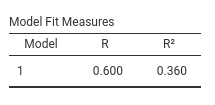
For arith the \(R^2\)
is the same found with PATHj, but for
read it is different. The reason is that the two
regressions do not consider the correlation between read
and arith, that cannot be included in the model and help to
explain variance. The path analysis model, instead, considers that
variance and incorporates it in the variance explained.
If we want to obtain with the path analysis the exact results
obtained with two regressions, we should set the correlation between
read and arith to zero, so the model would not
include it in the variance explained. We can do that by setting the
corresponding label (p6) to zero in the Custom Model Settings with the directive
p6==0.
 R-squared
 ───────────────────────────────────────────────────
   Variable    R²           Lower        Upper
 ───────────────────────────────────────────────────
   read        0.3516267    0.2840957    0.4186440
   arith       0.3600000    0.2924227    0.4268228
 ───────────────────────────────────────────────────
Results are now identical to the individual regressions. In other words, the advantage of a multivariate model over a series of individual univariate models is that the endogenous variables correlations are taken into the account in the former, and ignored in the latter. incidentally, a multivariate model with orthogonal (not correlated) dependent variables does not have any advantage over a series of univariate models.