PATHj computation details
keywords pathj,jamovi, path analyis ,interactions,categorical variables
PATHJ module details
PATHj version ≥ 0.5.* Draft version, mistakes may be around
Introduction
PATHj module estimation is based on
lavaan R package (Rosseel 2012). Most
of PATHj work is to prepare data and
options to be sent to lavaan, extract the output and pack it nicely for
jamovi output. Nonetheless, there are a few
operations that should be explained to let the user know what PATHj is actually doing. Here you find some
information.
Categorical Variables
PATHj accepts any categorical variable as exogenous variable, indepenently of the number of levels in the variable. This is achieved using a very general rule of linear models: any categorical variable can be cast in a linear model by representing it with K-1 contrast variables, where K is the number of levels.
Thus, when the user inserts a categorical variable in Exogenous Factors, PATHj creates K-1 new variables in the data sets, each representing a contrast between levels. What constrast weights are used is decided by the Factors Coding panel. All directives regarding the categorical variables (variances, regression coefficients, etc.) are applied to each contrast of the variable.
Generally speaking, this method works well. Here is an example:
Consider the data pathjexample, present in the module.
One categorical variable is called groups_a, featuring
three groups. If one uses R lm() to estimate the effect of
groups_a on y1, one gets the following
results:
library(pathj)
data("pathjdata")
model_formula<-y1~groups_a
pathjdata$groups_a<-factor(pathjdata$groups_a)
contrasts(pathjdata$groups_a)<-contr.treatment(3)-(1/3)  # centered constrasts with group 1 as reference group
summary(lm(model_formula,data=pathjdata))
##
## Call:
## lm(formula = model_formula, data = pathjdata)
##
## Residuals:
## Min 1Q Median 3Q Max
## -6.4601 -1.4179 -0.1222 1.3417 6.0651
##
## Coefficients:
## Estimate Std. Error t value Pr(>|t|)
## (Intercept) 0.1488 0.2318 0.642 0.522
## groups_a2 0.5305 0.5627 0.943 0.348
## groups_a3 0.2849 0.5579 0.511 0.611
##
## Residual standard error: 2.311 on 97 degrees of freedom
## Multiple R-squared: 0.009156, Adjusted R-squared: -0.01127
## F-statistic: 0.4481 on 2 and 97 DF, p-value: 0.6401If we know run the same model in PATHj, we get the same results in terms of coefficients and interpretation.
mod<-pathj::pathj(formula=list(model_formula),
                  data=pathjdata,
                  r2test = TRUE)
mod$models$r2
mod$models$coefficients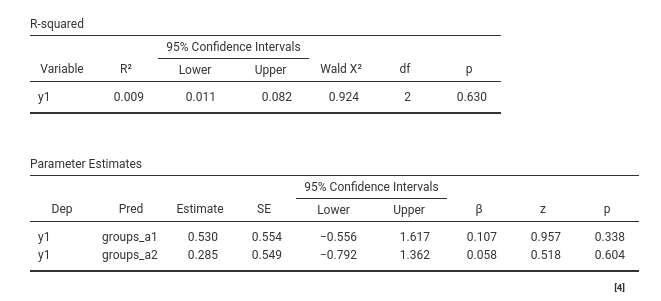
The coefficients are the same in R lm() and in PATHj. Standard errors are slightly different,
but that is due to the fact that regression uses OLS and path analysis
uses ML. We also get the same \(R^2\)
and comparable p-value for the \(R^2\),
which is discussed below .
Interactions
PATHj accepts interactions of any order. This is implemented by creating, for each interaction term, a new variable which is the product of the variables composing the interaction. The products are computed after any transformation of the variables (such as centering or standardizing), providing accurate estimation of the interaction coefficients.
The only side-effect of this method is that if an interaction term is present in more than one directive, it must be defined always with the same order of terms. As an example, the following model will fail in PATHj:
y1~x1+x2+x1:x2
y2~x1+x2+x2:x1
We fix this issue in R by simply defining the model as:
y1~x1+x2+x1:x2
y2~x1+x2+x1:x2
PATHj handles this issue in jamovi by ordering interaction terms alphabetically.
\(R^2\)
\(R^2\) are computed as one minus the standardized residual variance of each endogenous variable. Practically, defining \(\hat{\sigma}^2_r\) as the standardized residual variance, \(R^2_v=1-\hat{\sigma}^2_r\)
As regards the confidence intervals, by default they are estimated converting \(R^2\) to \(R\), then to \(z\) using the Fisher Z-transformation, then estimating the C.I. for \(z\) and back transform them to \(R^2\). The actual formula is in Carlson (2013), and is implemented as follows (R2 is the R-squared, N is the sample size, ciwidth is the C.I. width, usually .95):
      r<-sqrt(R2)
      f<-.5 * log((1 + r)/(1 - r))
      zr<-f*sqrt((N-3))
      z0<-qnorm((1-ciwidth)/2,lower.tail = F)
      lower<-zr-z0
      upper<-zr+z0
      flower<-lower/sqrt(N-3)
      fupper<-upper/sqrt(N-3)
      rupper<-(exp(2*fupper)-1)/(1+exp(2*fupper))
      rupper<-rupper^2
      rlower<-(exp(2*flower)-1)/(1+exp(2*flower))
      rlower<-rlower^2
The alternative method Residual C.I. employes the
residual variance C.I., by simply computing one minus the standardized
limits of the residual variance C.I.. This method may yield negative
lower bounds, which do not make much sense in the context of \(R^2\).
As regards the inferential tests associated with the \(R^2\)’s (option R-squared tests in Model Options panel), they are obtained as Wald’s chi-squared tests comparing the orginal model with a constrained model in which all paths leading to the endogenous variable are set to zero (except the intercept). The p-values obtained in this way are very close to the p-values one obtains with standard GLM F-tests.
Comments?
Got comments, issues or spotted a bug? Please open an issue on PATHj at github or send me an email
’