Multigroup models
(Marcello Gallucci)
keywords multigroup analysis, moderated mediation, path analysis, lavaan, categorical variables, interactions
Draft version, mistakes may be around
In this example we show examples of multigroup path analysis. We are going to employ a dataset meant to demostrate moderated mediation, so we can take this opportunity to show both very basic multigroup analyses and some more advanced application of the method.
Research data
Data represent a fictitious dataset present in the rosetta R
package. In the package, the data are named cpbExample
and it can be found here.
The data are about the attitudes and self-reported contra-productive behaviour (CPB) of employees of an organisation. The model behind these data predicts that feelings of procedural injustice may lead to cynicism and cynicism may lead to CPB. For our purposes, we can also note that these effects may be different across genders. Two genders are present in the dataset, male and female gender.
Simple model without gender
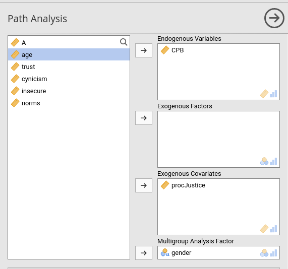
We start by fitting a simple model, with CPB as dependent variable
(endogenous) and procedural injustice (procJustice) as
independent variable (exogenous). In PATHj, we first set the variables role.

The relation between the independent and the dependent variables are
set in the Endogenous Models panel.

As soon as we set the model, the results appear on the right panel of
jamovi. For this example, it is interesting
to check the Estimates group of tables,
Parameters estimates in particular, which gives the simple
regression coefficients.
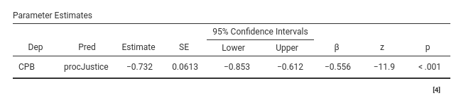
The coefficient linking procJustice to CPB
(here equal to -.732) is computed for the whole sample. We
now want to estimate this quantity in the two different genders and we
want to know whether the effect of procJustice on
CPB is different across genders.
For the first aim, we simple need to add gender into the
Multigroup Analysis Factor field.
and check the parameters estimates again.
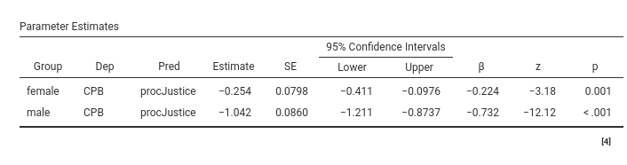
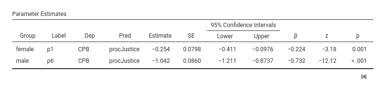
We can see that the estimates are presented by gender, so the effect
of procJustice on CPB is -.254
for female gender and 1.042 for male gender. In the table,
all results (CI and inferential tests) are replicated for the two
genders. Also the other tables in the results report estimates broken
down by gender. This basically means that we have split the model in two
submodels, one for women and one for man. It is a good idea to explore
the output and check all results, to assess possible differences between
the two groups defined by the factor variable.
We now want to test if the two coefficients -.254 and
1.042 are statistically significantly different. We can use
the standard approach used in path analysis of constraining two
parameters as equal, and evaluate the inferential test associated with
the constraint. The test (a \(Chi^2\))
is basically testing the misfit of the model due to the constraint, or,
more intuitively, is testing the null-hypothesis that the constraint is
true. In our case, it is testing that the two coefficients are the same
in the two groups.
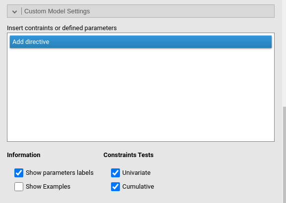
To obtain this test, we first go to
Custom Model Settings and ask for the show parameters labels
In the output, we see the same results as before, but now each
estimate has a label by which it can be uniquely identified. Our
estimates of interest are labeled p1 for female and
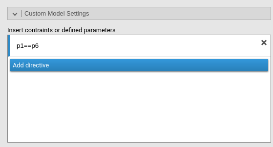
p6 for male gender. In the input, we click
Add directive in the Custom Model Settings and
declare the constraint p1==p6, that is the null-hypothesis
that we want to test.

As expected, the two coefficients p1 and p6
are now equal. The interesting table is the
Constraints Score Test, which gives us the inferential test
for the constraint we set.
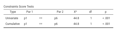
Here we find the test of the null-hypothesis described by the
constraint: We found a significant \(Chi^2\), so we can conclude that the two
coefficients are different. In general, this table provides one row for
each constraint set, marked as Univariate, and the
cumulative tests for all constraints together in the
Cumulative rows. Here, they are the same because we set
only one constraint.
With this technique, we can make all comparisons we want between groups, independently of the complexity of our model. Before that, however, it is worthwhile to give a more in-depth interpretation of the previous results, because it may help understanding how linear models work, over and beyond path analysis.
Multigroup tests and the General Linear Model
The first model we tests (wihout gender) was a simple regression that
can be obtained in jamovi with
Linear Regression command or with
General Linear Model in GAMLj module. Using the latter, we
obtain this.
It is easy to check that the estimate corresponds to the results we
obtained in PATHj. For some
applications, the inferential test may be slightly different, because
the GLM uses the t-test and PATHj
employs the z-test, but in this example they are the same
(11.9).
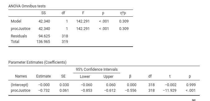
We can now add gender, and the interaction
gender*procJusting. The interaction, in the GLM, tests the
hypothesis that the effect of procJustice on
PBC is the same in both genders. Indeed, adding
gender and gender*procJusting in the GLM
yields:
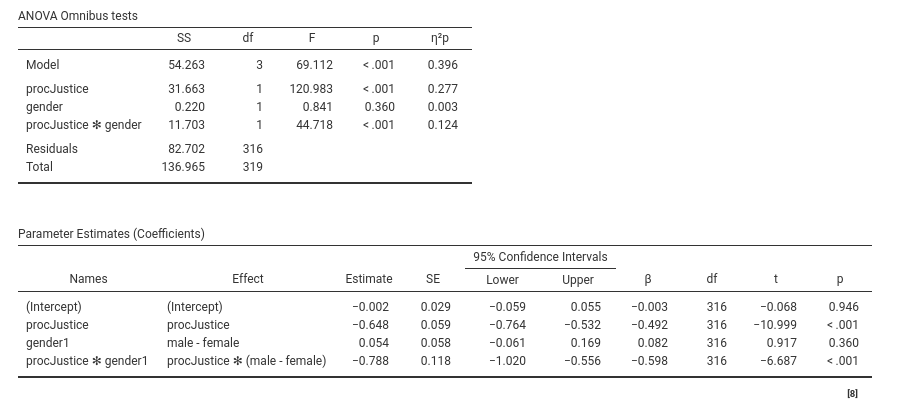
We can notice that the F-test associated with the interaction is
44.718, with pvalue less than .001, which is exactly the
same result we obtained in the Constraints Score Test
(\(Chi^2=F_{test}\) for \(df=1\)). Thus, when we tested the
multigroup constraint, we were actually testing the interaction
between the independent variable and the categorical variable set in the
multigroup factor. This means that whenever we have a categorical
variable in a path analysis, we can explore even complex interactions by
simply run a multigroup analysis, and set the appropriate
constraints.
What about the estimates we obtain when we set the multigroup
variable without constraints? We said that they were the estimates of
the effect of procJusting on CPB for the two
gender groups. In the GLM jargon, they are called Simple
Effects. Indeed, if we go to the GLM module and ask for the simple
effects, we get:
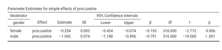
that correspond exactly to the estimtes given by PATHj. Thus, multigroup analysis estimates (without constraints) are the simple effects of the linear model, computed for each level of the multigroup variable. Constraining coefficients to be the same test interactions. Multigroup analysis is basically a moderation analysis.
More complex example
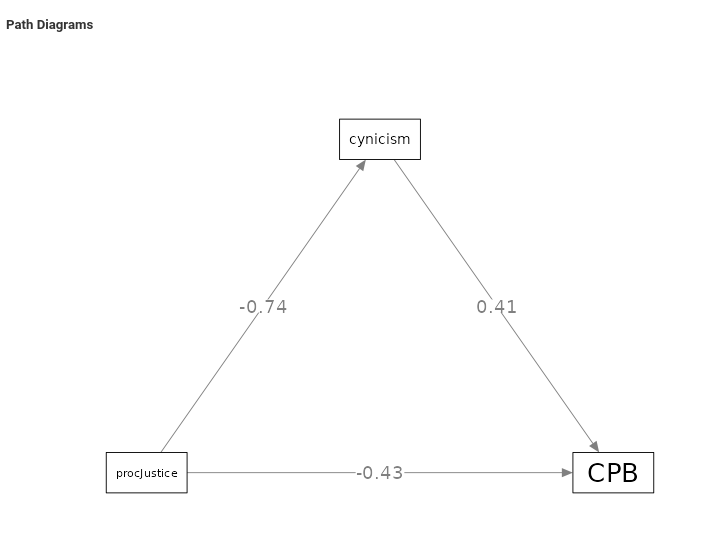
We now explore a more complex model, adding a mediator between
procedural justice and behavior. We add cynicism in the
Endogenous Variables field and let it predict
CPB and be predicted by procJustice. The model
(without gender) looks like this.
and it is set like this.

Because we are dealing with a mediation model, we can ask for the
Indirect Effects in the
Parameter Options panel.
This model gives average estimates of the relationship between the variables

and the average mediated effect.
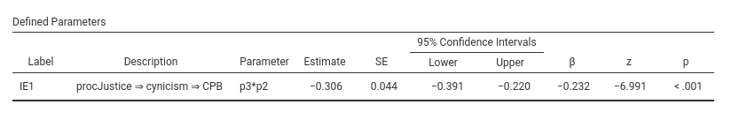
Thus, on average procJustice influences
cynicism (B=-.743, z=-11.12, p.<.001), which in turn
influences CPB (B=.411, z=8.99, p. <.001), yielding a
mediated effect of -.303, z=-6.991, p.<.001.
We now want to test wheter this mediated effect is present in each of
the gender groups, and if the mediated effect si different across
groups. Thus, we include gender as the
Multigroup Analysis Factor as we did before, and we obtain
the estimates broken down by gender.
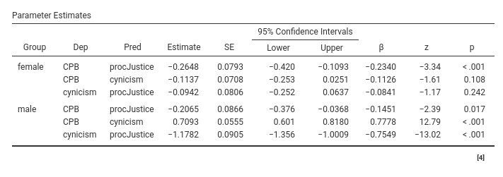
Thus, for female group, procJustice does not influence
significantly cynicism (B=-.094, z=-1.17, p.=242), which in
turn does not affect CPB (B=-.113, z=-1.61, p.=.108).
Coherently, the mediated effect is not appreciable and not statistically
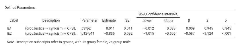
significant (ME=.011, z=.945, p.=.345). For male group, however, we find
that procJustice influences significantly
cynicism (B=-1.178, z=-13.02, p.<.001), which in turn
affects CPB (B=.709, z=12.79, p.<.001). The mediated
effect is thus statistically significant (B=-.836, z=-9.124,
p.<.001). Thus, we can say that cynicism seems to
mediate the effect of procJustice on CPB in
the male group but not in the female group.
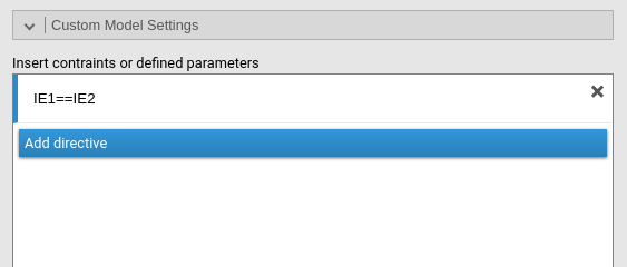
But do the mediated effects differ in the two groups? Establish that
two effects have different p-values in two groups it is not enough to
demonstrate that they are different. Thus, we need to test them. As
before, we simply go to Custom Model Settings and declare
the two mediated effects as equal, using the labels present in the
Indirect Effects table. Practically, we set
Now the indirect effects are estimated as equal across groups
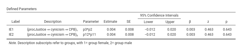
and the Constraints Score Tests gives us the test of the
difference of the two mediated effects.
We can conclude that the mediated effect are different in the two groups, thus we have a moderated mediation.
We can do more, though. We can probe the model asking why are they
different. A mediated effect is composed by at least two coefficients,
procJustice on cynicism (labelled
p3 and p12 for female and male group
respectively), and the effect of cynicism on
CPB (labelled p2 and p11 in the
tables). So, we can start asking whether the mediated effects are
different because the two groups are different in the size of the effect
of procJustice on cynicism, or because they
are different in the effect of cynicism on
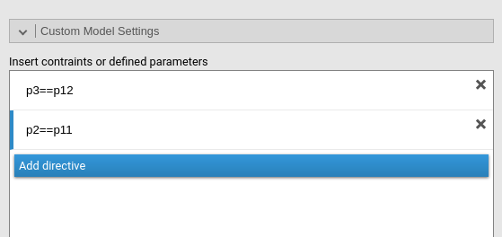
CPB, or both. To do that, we remove our previously set
constraint, and add p3==p12 and p2==p11 as a
new constraints.
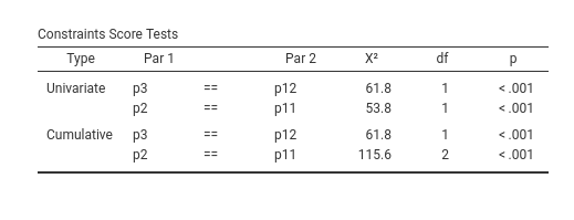
The chi-square testing the constraints signals that the two groups
are different in the firs leg of the mediation model,
procJustice on cynicism, with \(X^2(1)=61.8\) p.<.001 and in the second
leg, \(X^2(1)=53.8\), p.<.001.
Overall, the two constraints together are also significant \(X^2(2)=115.6\), p.<.001,
Because people tend to like bootstrap confidence intervals when they deal with mediation models, we can ask for the bootstrap confidence intervals of the mediated effects, in each groups (recall to remove the constraints otherwise the effects are computed as equal across groups), by going to `
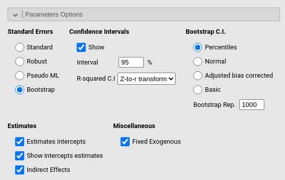
and the results will update giving the bootstrap confidence intervals.
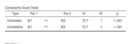
As a final touch, one can complete the analysis by adding the computation of the confidence interval (bootstrap or not) of the difference between the mediated effects. That could be useful for users who want to base their conclusions only on bootstrap inference. Well, just keep in mind that the difference between mediated effects it is just a defined parameter of the model, defined as the difference between the two defined parameters IE1 and IE2. We can set that explicitly in the model. However, we should use the coefficient labels, not the IE* labels. Notice in the results without constraints
the two mediated effects are given by p3*p2 for female
group and p12*p12 for the male group. They difference would
than be

and the Defined parameters table would now offer the
confidence intervals.

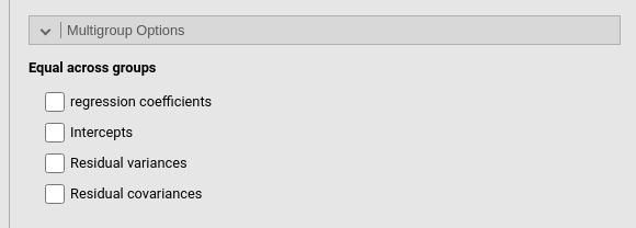
Additional Options
In the Multigroup Options panel, one can find a series
of options to bulk setting all coefficients of one type equal across
groups.
They are useful when large models are tested, even though setting the
appropriate constraints one by one in the
Custom Model Settings helps keeping the analysis under the
user control.